Scalar, 2D{1} datasets¶

The 2D{1} datasets are two dimensional, \(d=2\), with one single-component dependent variable, \(p=1\). Here, we present examples of 2D{1} datasets with the scalar dependent variable.

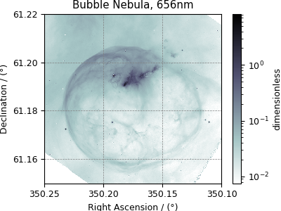
Astronomy dataset¶

The following dataset is a new observation of the Bubble Nebula acquired by The Hubble Heritage Team, in February 2016. The original dataset was obtained in the FITS format and subsequently converted to the CSD model file-format. For the convenience of illustration, we have downsampled the original dataset.

Let’s load the .csdfe file and look at its data structure.

>>> import csdmpy as cp
>>> bubble_nebula = cp.load('Test Files/BubbleNebula/Bubble.csdfe')
>>> print(bubble_nebula.data_structure)
{
  "csdm": {
    "version": "1.0",
    "read_only": true,
    "timestamp": "2016-02-26T16:41:00Z",
    "description": "The dataset is a new observation of the Bubble Nebula acquired by The Hubble Heritage Team, in February 2016.",
    "dimensions": [
      {
        "type": "linear",
        "count": 1024,
        "increment": "-0.0002581136196 °",
        "coordinates_offset": "350.311874957 °",
        "quantity_name": "plane angle",
        "label": "Right Ascension"
      },
      {
        "type": "linear",
        "count": 1024,
        "increment": "0.0001219957797701109 °",
        "coordinates_offset": "61.12851494969163 °",
        "quantity_name": "plane angle",
        "label": "Declination"
      }
    ],
    "dependent_variables": [
      {
        "type": "internal",
        "name": "Bubble Nebula, 656nm",
        "numeric_type": "float32",
        "quantity_type": "scalar",
        "components": [
          [
            "0.0, 0.0, ..., 0.0, 0.0"
          ]
        ]
      }
    ]
  }
}

Here, the variable bubble_nebula is an instance of the CSDM class. From the data structure, one finds two dimensions, labeled as Right Ascension and Declination, and one single-component dependent variable named Bubble Nebula, 656nm.

Let’s get the tuples of the dimension and dependent variable instances from the bubble_nebula instance following,

>>> x = bubble_nebula.dimensions
>>> y = bubble_nebula.dependent_variables

There are two dimension instances in x. Let’s look at the coordinates along each dimension, using the coordinates attribute of the respective instances.

>>> print(x[0].coordinates[:10])
[350.31187496 350.31161684 350.31135873 350.31110062 350.3108425
 350.31058439 350.31032628 350.31006816 350.30981005 350.30955193] deg

>>> print(x[1].coordinates[:10])
[61.12851495 61.12863695 61.12875894 61.12888094 61.12900293 61.12912493
 61.12924692 61.12936892 61.12949092 61.12961291] deg

Here, we only print the first ten coordinates along the respective dimensions.

The component of the dependent variable is accessed through the components attribute.

>>> y00 = y[0].components[0]

Visualizing the dataset

Now, to plot the dataset.

Tip

Intensity plot.

>>> import matplotlib.pyplot as plt
>>> from matplotlib.colors import LogNorm
>>> import numpy as np

>>> def plot():
...     # Figure setup.
...     fig, ax = plt.subplots(1,1, figsize=(4,3))
...     ax.set_facecolor('w')
...
...     # the coordinates along the two dimensions
...     x0 = x[0].coordinates
...     x1 = x[1].coordinates
...
...     # Set the extents of the image.
...     extent=[x0[0].value, x0[-1].value, x1[0].value, x1[-1].value]
...
...     # Log intensity image plot.
...     im = ax.imshow(np.abs(y00), origin='lower', cmap='bone_r',
...                    norm=LogNorm(vmax=y00.max()/10, vmin=7.5e-3, clip=True),
...                    extent=extent, aspect='auto')
...
...     # Set the axes labels and the figure tile.
...     ax.set_xlabel(x[0].axis_label)
...     ax.set_ylabel(x[1].axis_label)
...     ax.set_title(y[0].name)
...     ax.locator_params(nbins=5)
...
...     # Add a colorbar.
...     cbar = fig.colorbar(im)
...     cbar.ax.set_ylabel(y[0].axis_label[0])
...
...     # Set the x and y limits.
...     ax.set_xlim([350.25, 350.1])
...     ax.set_ylim([61.15, 61.22])
...
...     # Add grid lines.
...     ax.grid(color='gray', linestyle='--', linewidth=0.5)
...
...     plt.tight_layout(pad=0, w_pad=0, h_pad=0)
...     plt.show()

>>> plot()

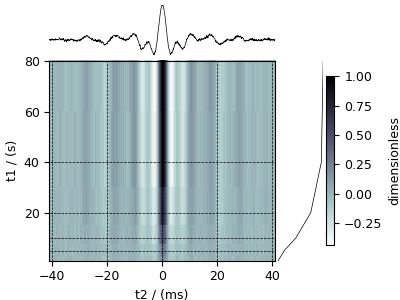
Nuclear Magnetic Resonance (NMR) dataset¶

The following example is a \(^{29}\mathrm{Si}\) NMR time-domain saturation recovery measurement of a highly siliceous zeolite ZSM-12. Usually, the spin recovery measurements are acquired over a rectilinear grid where measurements along one of the dimensions are non-uniform and span several orders of magnitude. In this example, we illustrate the use of monotonic dimensions for describing such datasets.

Let’s load the file.

>>> import csdmpy as cp

>>> filename = 'Test Files/NMR/satrec/satRec.csdf'
>>> NMR_2D_data = cp.load(filename)

The tuples of the dimension and dependent variable instances from the NMR_2D_data instance are

>>> x = NMR_2D_data.dimensions
>>> y = NMR_2D_data.dependent_variables

respectively. There are two dimension instances in this example with respective dimension data structures as

>>> print(x[0].data_structure)
{
  "type": "linear",
  "description": "A full echo echo acquisition along the t2 dimension using a Hahn echo.",
  "count": 1024,
  "increment": "80.0 µs",
  "coordinates_offset": "-41.04 ms",
  "quantity_name": "time",
  "label": "t2",
  "reciprocal": {
    "coordinates_offset": "-8766.0626 Hz",
    "origin_offset": "79578822.26200001 Hz",
    "quantity_name": "frequency",
    "label": "29Si frequency shift"
  }
}

and

>>> print(x[1].data_structure)
{
  "type": "monotonic",
  "coordinates": [
    "1 s",
    "5 s",
    "10 s",
    "20 s",
    "40 s",
    "80 s"
  ],
  "quantity_name": "time",
  "label": "t1",
  "reciprocal": {
    "quantity_name": "frequency"
  }
}

respectively. The first dimension is uniformly spaced, as indicated by the linear subtype, while the second dimension is non-linear and monotonically sampled. The coordinates along the respective dimensions are

>>> x0 = x[0].coordinates
>>> print(x0)
[-41040. -40960. -40880. ...  40640.  40720.  40800.] us

>>> x1 = x[1].coordinates
>>> print(x1)
[ 1.  5. 10. 20. 40. 80.] s

Notice, the unit of x0 is in microseconds. It might be convenient to convert the unit to milliseconds. To do so, use the to() method of the respective Dimension instance as follows,

>>> x[0].to('ms')
>>> x0 = x[0].coordinates
>>> print(x0)
[-41.04 -40.96 -40.88 ...  40.64  40.72  40.8 ] ms

As before, the components of the dependent variable are accessed using the components attribute.

>>> y00 = y[0].components[0]
>>> print(y00)
[[  182.26953   +136.4989j    -530.45996   +145.59097j
   -648.56055   +296.6433j   ... -1034.6655    +123.473114j
    137.29883   +144.3381j    -151.75049    -18.316727j]
 [  -80.799805  +138.63733j   -330.4419    -131.69786j
   -356.23877   +463.6406j   ...   854.9712    +373.60577j
    432.64648   +525.6024j     -35.51758   -141.60239j ]
 [ -215.80469   +163.03308j   -330.6836    -308.8578j
  -1313.7393   -1557.9144j   ...  -979.9209    +271.06757j
   -667.6211     +61.262817j   150.32227    -41.081024j]
 [    6.2421875 -163.0319j    -654.5654    +372.27518j
  -1209.3877    -217.7103j   ...   202.91211   +910.0657j
   -163.88281   +343.41882j     27.354492   +21.467224j]
 [  -86.03516   -129.40945j   -461.1875     -74.49284j
     68.13672   -641.11975j  ...   803.3242    -423.6355j
   -267.3672    -226.39514j     77.77344    +80.2041j  ]
 [ -436.0664    -131.52814j    216.32812   +441.56696j
   -577.0254    -658.17645j  ... -1780.457     +454.20862j
  -1765.7441    -375.72888j    407.0703    +162.24716j ]]

Visualizing the dataset

Tip

Intensity plot with cross-sections

More often than not, the code required to plot the data become exhaustive. Here is one such example.

>>> import matplotlib.pyplot as plt
>>> from matplotlib.image import NonUniformImage
>>> import numpy as np

>>> def plot_nmr_2d():
...     """
...     Set the extents of the image.
...     To set the independent variable coordinates at the center of each image
...     pixel, subtract and add half the sampling interval from the first
...     and the last coordinate, respectively, of the linearly sampled
...     dimension, i.e., x0.
...     """
...     si=x[0].increment
...     extent = ((x0[0]-0.5*si).to('ms').value,
...               (x0[-1]+0.5*si).to('ms').value,
...               x1[0].value,
...               x1[-1].value)
...
...     """
...     Create a 2x2 subplot grid. The subplot at the lower-left corner is for
...     the image intensity plot. The subplots at the top-left and bottom-right
...     are for the data slice at the horizontal and vertical cross-section,
...     respectively. The subplot at the top-right corner is empty.
...     """
...     fig, axi = plt.subplots(2,2, figsize=(4,3),
...                             gridspec_kw = {'width_ratios':[4,1],
...                                            'height_ratios':[1,4]})
...
...     """
...     The image subplot quadrant.
...     Add an image over a rectilinear grid. Here, only the real part of the
...     data values is used.
...     """
...     ax = axi[1,0]
...     im = NonUniformImage(ax, interpolation='nearest',
...                          extent=extent, cmap='bone_r')
...     im.set_data(x0, x1, y00.real/y00.real.max())
...
...     """Add the colorbar and the component label."""
...     cbar = fig.colorbar(im)
...     cbar.ax.set_ylabel(y[0].axis_label[0])
...
...     """Set up the grid lines."""
...     ax.images.append(im)
...     for i in range(x1.size):
...         ax.plot(x0, np.ones(x0.size)*x1[i], 'k--', linewidth=0.5)
...     ax.grid(axis='x', color='k', linestyle='--', linewidth=0.5, which='both')
...
...     """Setup the axes, add the axes labels, and the figure title."""
...     ax.set_xlim([extent[0], extent[1]])
...     ax.set_ylim([extent[2], extent[3]])
...     ax.set_xlabel(x[0].axis_label)
...     ax.set_ylabel(x[1].axis_label)
...     ax.set_title(y[0].name)
...
...     """Add the horizontal data slice to the top-left subplot."""
...     ax0 = axi[0,0]
...     top = y00[-1].real
...     ax0.plot(x0, top, 'k', linewidth=0.5)
...     ax0.set_xlim([extent[0], extent[1]])
...     ax0.set_ylim([top.min(), top.max()])
...     ax0.axis('off')
...
...     """Add the vertical data slice to the bottom-right subplot."""
...     ax1 = axi[1,1]
...     right = y00[:,513].real
...     ax1.plot(right, x1, 'k', linewidth=0.5)
...     ax1.set_ylim([extent[2], extent[3]])
...     ax1.set_xlim([right.min(),  right.max()])
...     ax1.axis('off')
...
...     """Turn off the axis system for the top-right subplot."""
...     axi[0,1].axis('off')
...
...     plt.tight_layout(pad=0., w_pad=0., h_pad=0.)
...     plt.subplots_adjust(wspace=0.025, hspace=0.05)
...     plt.show()

>>> plot_nmr_2d()

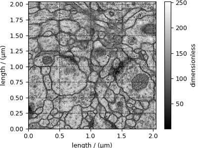
Transmission Electron Microscopy (TEM) dataset¶

The following TEM dataset is a section of an early larval brain of Drosophila melanogaster used in the analysis of neuronal microcircuitry. The dataset was obtained from the TrakEM2 tutorial and subsequently converted to the CSD model file-format.

Let’s import the CSD model data-file and look at its data structure.

>>> import csdmpy as cp
>>> import matplotlib.pyplot as plt

>>> filename = 'Test Files/TEM/TEM.csdf'
>>> TEM = cp.load(filename)
>>> print(TEM.data_structure)
{
  "csdm": {
    "version": "1.0",
    "read_only": true,
    "timestamp": "2016-03-12T16:41:00Z",
    "description": "TEM image of the early larval brain of Drosophila melanogaster used in the analysis of neuronal microcircuitry.",
    "dimensions": [
      {
        "type": "linear",
        "count": 512,
        "increment": "4.0 nm",
        "quantity_name": "length",
        "reciprocal": {
          "quantity_name": "wavenumber"
        }
      },
      {
        "type": "linear",
        "count": 512,
        "increment": "4.0 nm",
        "quantity_name": "length",
        "reciprocal": {
          "quantity_name": "wavenumber"
        }
      }
    ],
    "dependent_variables": [
      {
        "type": "internal",
        "numeric_type": "uint8",
        "quantity_type": "scalar",
        "components": [
          [
            "126, 107, ..., 164, 171"
          ]
        ]
      }
    ]
  }
}

This dataset consists of two linear dimensions and one single-component dependent variable. The tuples of the dimension and the dependent variable instances from this example are

>>> x = TEM.dimensions
>>> y = TEM.dependent_variables

and the respective coordinates (viewed only for the first ten coordinates),

>>> print(x[0].coordinates[:10])
[ 0.  4.  8. 12. 16. 20. 24. 28. 32. 36.] nm

>>> print(x[1].coordinates[:10])
[ 0.  4.  8. 12. 16. 20. 24. 28. 32. 36.] nm

For convenience, let’s convert the coordinate from nm to µm using the to() method of the respective Dimension instance,

>>> x[0].to('µm')
>>> x[1].to('µm')

and plot the data.

>>> def plot_image():
...     plt.figure(figsize=(4,3))
...
...     # Set the extents of the image plot.
...     extent = [x[0].coordinates[0].value, x[0].coordinates[-1].value,
...               x[1].coordinates[0].value, x[1].coordinates[-1].value]
...
...     # Add the image plot.
...     im = plt.imshow(y[0].components[0], origin='lower', extent=extent, cmap='gray')
...
...     # Add a colorbar.
...     cbar = plt.gca().figure.colorbar(im)
...     cbar.ax.set_ylabel(y[0].axis_label[0])
...
...     # Set up the axes label and figure title.
...     plt.xlabel(x[0].axis_label)
...     plt.ylabel(x[1].axis_label)
...     plt.title(y[0].name)
...
...     # Set up the grid lines.
...     plt.grid(color='k', linestyle='--', linewidth=0.5)
...
...     plt.tight_layout(pad=0, w_pad=0, h_pad=0)
...     plt.show()

>>> plot_image()

Table of Contents

Previous topic

Next topic

This Page

Scalar, 2D{1} datasets¶

Astronomy dataset¶

Nuclear Magnetic Resonance (NMR) dataset¶

Transmission Electron Microscopy (TEM) dataset¶